The pictures are here!!!

A couple of weeks ago I received a zip file that contained pictures taken in the arctic.  They were very neatly organized in dated folders.  I received pictures from two cameras.  One of them was intended to test a special InfraRed filter (IR).  The other was used to test the usefulness of the cmucam3 camera for our specific purposes.  I will refer to the second batch of pictures.  The InfraRed filter pictures I have not analyzed yet.

Lars (Our friendly biologists :) separated the pictures into different distance groups.  There were three: 100cm, 70cm and 40cm.  He chose two plots to take pictures of.  Each time he photographed a plot, he took 6 pictures (two of each distance).  He did a really good job at tagging the images.

We were looking at how the camera behaves in terms of focus, resolution and general survivability.  I was told that the cameras did well in terms of battery life and they basically worked as they were supposed to.  I also received feedback in terms of camera usability.  There were three comments that I want to highlight: 1. It is difficult to focus the pictures without an image feedback, 2. Sometimes the pictures did not take, 3. The resolution is very low to do any kind of annotations.  I have already added these comments to the issues in the project page.  There I have possible solutions for each issue.

This is the picture taken from 100cm.  One can barely notice anything.  There are also some black regions and red and white pixels that are probably some sort of issue in the imager.  Also notice that, while one cannot differentiate details, one can detect  patches of activity.  From this picture one could have an informed guess as to where the flowers might or might not be located.  Patches of gray might indicate that there is no vegetation activity.  Of course this depends on the type of flower we are studying.  But my point is that this picture gives information!  Also notice that one can see the plot separators in this image.

In the picture on the right the image gets a bit closer.  Its taken from a height of 70cm. Not a lot of detail is revealed to use, compared to the previous image.  We can see that the plot separator is more noticeable.  We can’t see the others because the picture is taken close to the plot.  We do however start to notice some shapes.  We recognize the bigger leaves in the top right and in the bottom left of the image.  As with the previous image, we can also see a bunch of red pixels, don’t really know where they come from.
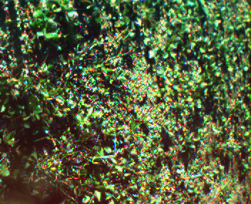
The image on the left is taken from a height of 30cm.  In this one we can make out some leaves and some stems running along the ground.  We can’t, however, make out any flowers.  Notice also that there are red pixels sprinkled all over the place.

The general feeling is that the resolution is way to low to do any kind of detecting or annotating.  Seeing these pictures I have to agree.  I cannot see how we can directly detect the flowers from these pictures. But we can use these imagers as the first line of detection.  They can tell us where the flowers are and we can point the other more powerful imagers in that particular direction.  In general I don’t want to dismiss these cameras just yet.

I’m working on a new camera that will have double the resolution.  Hopefully this will get us to a point were we can see some flowers.

Posted in PhD, wireless image sensor networks | Leave a comment

The convert command. Nice!

I’ve actually used this command before but today I was pleasantly surprised.  I had used it in the past to change from one image format to another.  It’s actually very straight forward and it helps a bunch when you just want an easy way to convert images.  You can change the extensions of the files to signify what type of image you want to convert to.

convert in.jpg out.png

Today I wanted to do something a bit different.  I wanted to rapidly re-size a bunch of images I had in a directory.  As with the last case I wanted to avoid opening up gimp and manually changing all the images.  I know that you can do it in gimp with python and other scripting languages, but it seems overkill for me.  I revisited the `convert` command and it gave me the solution that I was searching.

convert in.jpg -resize GEOMETRY out.jpg

GEOMETRY in this case can be a lot of things.  I used two flavors of this argument.  You can either define the height and width of the image or the percentage of resizing.  If you want to define the height and the width you use ‘x’ to separate the two values:

convert in.jpg -resize 40x40 out.jpg

This is cool if you know exactly what dimensions you want out of your resulting image.  In my case I just wanted the image to shrink by a certain ratio.  This is where the command surprised me :).  One can also define the GEOMETRY as a percentage.  when the percentage is more than 100, it means that the image is going to increase in size.  If the percentage is 100, then the image will not be re-sized (I think it’s not touched).  Finally, when the percentage is less than 100, the image shrinks.  I used the command in the following manner:

convert in.jpg -resize 30% out.jpg

This is really convenient for me because I can just use a shell `for` to traverse all my images:

for file in *; do convert $file -resize 30% smaller-$file; done ;
Posted in commands | Leave a comment

Back of the envelope: Remember! There is a compiler.

Thx to my adviser I realized that there is a compiler translating the stuff that I code.  This becomes extremely relative when you are trying to time certain things.  Is the compiler really translating the code that I write to an executable that does exactly the same thing that I told it to do? Or does it think it’s better than me? :)

When I looked at Philippe’s (My adviser) java code, I realized that he had used a static variable outside the functions as the destination of the operation.  When I asked him for the reason of his decision, he answered: “If you were a compiler, and you saw a loop get executed many times to do exactly the same and the results is thrown away. What would you do?”.  I immediately realized my potential mistake and went back to the code :).  I now have two different files that I have analyzed.  One is the previous C file with some changes.  And the other is a modification of the java file that Philippe gave me [1],[2].

The following are my results when I run the commands in my machine.  I know little about what the compiler does in these cases.  With that said, the output of the commands is very…. interesting :)

The result from the C code:

[joel@jogr temp]$ gcc temp.c -O0 -o operations
[joel@jogr temp]$ ./operations 1000000000
Global variable
Add: 1890.000000 ms
Mul: 3030.000000 ms
Div: 6880.000000 ms
Local variable
Add: 2110.000000 ms
Mul: 3040.000000 ms
Div: 6900.000000 ms
[joel@jogr temp]$ gcc temp.c -O2 -o operations
[joel@jogr temp]$ ./operations 1000000000
Global variable
Add: 0.000000 ms
Mul: 540.000000 ms
Div: 4230.000000 ms
Local variable
Add: 0.000000 ms
Mul: 0.000000 ms
Div: 0.000000 ms

These results differ from the ones I posted in my first “Back of the envelope” post.  Notice that I not only changed the code to use a global var, but I also used to different compilation options.  We see here that gcc (the compiler that I used) thinks it’s really smart when used with -O2.  When it sees that I used a local variable in my for loops, it just ignored it completely.  When using a global variable it “thinks twice” about optimizing the for loop completely out and chooses something else.  Though the use of a global variable seems to be faster.

The result from the Java code:

[joel@jogr temp]$ javac C.java
[joel@jogr temp]$ java C  1000000000
Global vars:
Add: 750 ms
Mul: 1688 ms
Div: 2317 ms
Local vars
Add: 745 ms
Mul: 746 ms
Div: 744 ms
[joel@jogr temp]$

I didn’t find any optimizing option that I could use with javac, so I chose to just run it one time.  Here we see clearly that my java compiler thinks it’s really smart too.  When it sees that I’m using local variables it is faster than when I use a global variable.  This probably means that it is somehow optimizing stuff under the hood.

It is curious (to me) how much faster java is.  I confess that I don’t know lots of things that happen in the java and C compilation processes.  But I still would have thunk that, out of these two files, C would have come out on top.  I guess you never stop surprising yourself :)  That’ll teach me to pick on java :)

Would love to hear what happened when you tried it!!! Leave a comment with your results or if you see that I did something completely idiotic :)

[1] http://www.itu.dk/people/jogr/classes/SDBS/FALL2010/20100908operations.c
[2] http://www.itu.dk/people/jogr/classes/SDBS/FALL2010/20100908C.java
Posted in PhD | Leave a comment

gmail: filter attachment names and auto responses

Searching for a way to better the current way of receiving assignments (We should probably be using something like egroupware for universities, one can dream) I stumbled upon some nifty tricks to make life that much easier.

The issue came when I wanted to create a filter that analyzed the attachment file name.  I found out that one can use the keywork “filename:” together with the checkbox “has attachment”.  Therefore if one wants to act when receiving a mail that contains a pdf attachment, one needs to check the “has attachment” checkbox and the type “filename: pdf” in the “Has the words” text area.  There is a downside to this approach: if the sender attached a file that ends in “.pdf” and the file is not actually a pdf, it will match it anyway.  In other words the Gmail code does not actually check the mail, but just the name.

After I identified the emails that came in and had pdf attachments I wanted to auto-respond to them.  When I went to create an action for the filter, no action had the auto-respond mechanism that I was looking for, so I googled a bit.  After some searching I came across something called “Canned response”.  This is basically a predefined mail that e-mail keeps somewhere and you can use it when defining an action in a filter or when answering an incoming mail.  To use this feature I had to activate the Gmail lab called “Canned responses”.

This is probably one of the things that bothered me the most of the Gmail filters.  The fact that one could not have a smaller granularity with one’s information.  Now that I have discovered tagged filters, I like Gmail a bit more.

Posted in commands | Leave a comment

Back of the envelope.

Was reading Jon Bentley Programming Perls (second edition) [1] and  I don’t feel particularly good confessing that I had not read this book before.  It has lots of really nice programming tidbits that can be very helpful in the day-2-day.  The book is a compilation of columns that appeared in one of the ACMs publications.  Therefore it is organized in chapters that directly reflect the columns that appeared in the ACM.

I received an activity for the class that I will TA this semester.  The activity is centered in one of the chapters of Programming Perls: Back of the envelope calculations (BOEC).  In general these are quick processes that do not have to be exact and are made to make decision about a certain process.  Jon Bentley has really nice examples of situations were he has used back of the envelope calculations.  These examples are taken from real life situations that prove their importance.

The activity [2] that was given to me contains two main points: I assume that the first is intended as a warm-up activity that will lead into the second part; the second is made up of 3 curious exercises that taught me the importance of BOEC.  I basically ignored the first part and concentrated my efforts in the second section.  The first two I did in about 15 mins.  I did the calculations in my notebook and modified the values a little to make the calculations easier.  So if I had to divide by 3600, I chose to divide by 3000 (I’m lazy).  After digesting the results a little and double checking them, I continued and calculated everything with the exact values.  I used the calc command [3].  I then compared the results from my approximate calculations with the “correct” ones.  The “correct” calculations were not 100% correct as one has to assume things like average bike velocity.

What I saw when comparing the approximate value and the “correct” value was that, though they were different, their values fell into the same ball park.  That means that I would have taken the same decision based on the approximate values than on the “correct” values.  the approximate values being much faster to calculate.  In general this is a very good way to give a first tier validation to whatever you are doing.  Not happy with what I learned I coded a little script that shows exactly what I did for the first two exercises [4].

For the third exercise I just created a python script and some C code to get some numbers out.  After running them on my  box I got the following results.

For PYTHON:
1 addition in 0.00966 secs
1 subtraction in 0.00857 secs
1 division in 0.023 secs
1 multiplication in 0.0089 secs

For C: ran with argument 1000000000
1 addition in 2.62e-9
1 subtraction in 2.64r-9
1 division in 2.64e-9
1 multiplication in 2.62e-9

This is a primitive comparison of language performance.  Though this is not intended to be an accurate benchmark for integer operations, It gives us some information:  Like the fact that python will probably run 10e6 times slower than C when operating.  Or that C gets really close to an operation per cycle.  It takes a bit less than the advertised velocity for one core in my box.  And finally, python was much easier to code than C :)

[1] http://www.amazon.co.uk/Programming-Pearls-ACM-Press-Bentley/dp/0201657880/ref=sr_1_1?ie=UTF8&s=books&qid=1283767271&sr=8-1
[2] http://www.itu.dk/people/jogr/classes/SDBS/FALL2010/20100906BackOfTheEnvelopPuzzles.pdf
[3] http://isthe.com/chongo/tech/comp/calc/
[4] http://www.itu.dk/people/jogr/classes/SDBS/FALL2010/20100906botep.sh
[5] http://www.itu.dk/people/jogr/classes/SDBS/FALL2010/20100906operations.c
[6] http://www.itu.dk/people/jogr/classes/SDBS/FALL2010/20100906operations.py
Posted in PhD | Leave a comment

Image adjust, Its working!!!

Finally got a working command out of my opencv experiment.  I still need to work on some additional aspects.  but the overall src is already finished.  I ended up with 3 major states for the command:

  1. video_demo:  This state shows the capability of the imageadjust command in a video.  I thought it would be nice to see it real-time with a feed from the camera of from a video file.  It’s very cool to compare the original video feed with the changed image.  ./imageadjust –cw # –ch # –video_demo [–video FILE | -c 0].
  2. create_conf: Its used to create the configuration file from a series of pictures, a video file or a video feed.  This is good because (i thing) the command runs faster when you give it the configuration parameters.  It all depends on opencv internals that I don’t understand quite yet.  ./imageadjust –cw # –ch # –create_conf [IMAGES | -c 0 | –video FILE ]
  3. image_adjust: It’s the main objective of the command.  You give it a list of images and, optionally, a configuration file.  And it will create a directory and put all the adjusted images there.  For the moment there is a bug related with the configuration file code.  So the resulting images when executing the command with –ininput is not so good.  The angle of the images is not adjusted correctly.  Will fix that shortly :)

At the end the distance and angle are adjusted to an undefined position.  That is, the use cannot define the resulting angle nor distance.  This could be something that can be added in the future, but I’m happy with the way things are for the moment.  The distance is defined by the largest distance from the image plane of the list of images.  It means that all the images will be adjusted to have the distance of the image with the most distance from the camera.  Not really sure what the angle is.  On all the images the chessboard ends up with the longest side in the vertical position.

Going to fix the remaining outstanding issues and start using the command tomorrow :)

This is the git snapshot:

http://github.com/Joelgranados/imageadjust/tree/94028b5dad9a46b690b75d185cbc77153a86b695
Posted in opencv, PhD | Leave a comment

Paper: Reducing Power Consumption of Image Transmission over IEEE 802.15.4/ZigBee Sensor Network

Topic of interest: Energy consumption of image transmission in Wireless Sensor Networks.

Approach: “Power reduction while transmitting images in WSN over IEEE 802.15.4/ZigBee by disabling MAC acks”.  Some additional control messages needed to be implemented in the application layer.

year: 2010

Findings:

  1. They where able to calculate a a 7.6% reduction on a coordinator and end device.
  2. They also calculated 1.6% active time reduction in both coordinator and end device.

Comments:

  1. I finally found the accepted name for these types of WSN -> Wireless Image Sensor Networks (WiSNs).  Seems obvious, but it’s not so much when you don’t know the term.
  2. The tests are performed indoors and at a rather close range.  A question remains of what type of interference was present in the indoor environment. Additionally I ask myself if there are other factors of interference when the WiSN is taken to the field.
  3. I wonder how much the results (throughput, BER, PER) suffer when the tests are done outdoors.
  4. This work is done to increment the efficiency of the ZigBee protocol.  I wonder if it not easier to use another protocol.

link: http://ieeexplore.ieee.org/stamp/stamp.jsp?tp=&arnumber=5488204

Posted in papers, PhD, wireless image sensor networks | Leave a comment

Dagstuhl 2010, Conet summer school

I spent this week in the Conet 2010 summer school in Dagstuhl.  I beautiful place in the german mid-west.  The first days were a bit rainy, but the weather got better at the end.  This place is like the computer scientists heaven.  There is a library here with journals that date back to as far as 1958.  And they also have an archive (that I did not visit) that might hold more interesting stuff.  I found myself reading an IEEE Computer article from the early 60 that talked about how computers were starting to get too fast.  And how that increase was changing the way programmers interacted with them.  It was funny and gave me a sort of perspective.

For the first 3 days the summer school was organized in one and a half hour sessions given by well renowned professors.  On Wednesday we had some short presentations from PhD students that were describing their findings or talked about the objectives that they had for their yet to be completed projects.  Finally on Thursday and Friday we had two hands-on tutorials and additional presentations.  There are a couple of presentations on Saturday that I will unfortunately not attend.

Of the presentations I have to highlight the one that John Stancovic gave at the beginning of the summer school.  It was actually the opening presentation.  There was one thing that I noticed among the things that he touched in his presentation.  He gave a special place to the importance of robustness in cyber physical systems.  This is something that I have had in the back of my mind since I started my PhD, but it acquired a new light when it was mentioned by Prof. Stankovic.  Though it was jus t a small part of his overall presentation, it was something that I noticed and gave me a bit of direction in my work. [1]

Another highlight of the presentations was the intelligent window by Hartmut Hillmer.  His talk did not really overlap on my work on reliability on WSN, but it was witty and very expressive.  It was a breath of fresh air in a series of talks that were rapidly becoming monotonous.  His talk was centered in micromachining foundations and a window that used this technology to control sunlight use in indoor environments (among other things) [2].  I really liked it because of the way he explained concepts (used props and took various physical examples to the talk) and because he gave a wide overview of a field that I know very little about.

I also liked the talk given by Peter Cork about the work he has done throughout his career.  It gave a nice spectrum of the possibilities for WSN.  Though his talk was mainly based on robotics, most of his projects touched in some way or another on WSN. He did raise some interesting questions about some underlying assumptions that the general WSN community has had for a long time.  Mainly he questioned the overall consensus that embedded systems have very limited resources.  As I understood it, he didn’t actually want to say that embedded systems  have plentiful resource, but that in some occasions the whole thing gets  gets blown out of proportions.  And with the advent of new devices, its worth revisiting and assessing just how constraint the resources are.  This gives me hope in my search because we plan to use image recognition (notoriously resource hungry)  in embedded systems.

I met loads of people with very interesting opinions that come from all over the world and have all sorts of backgrounds.  I think this was the objective of the summer school and outweighed the presentations considerably.  First, the fact that I repeated what I was doing and what I intended to do more than a dozen times made me think about my work  and its final objective.  My peers did not notice but I was actually asking myself if what I was saying had an actual future and if it had a niche in the whole WSN community.  It was a very prolific exercise.  Though I am still far away from actually molding what I am doing into a research question, today I feel that much closer :)

I leave Dagstuhl filled with a sense of hope and new found energy.  i also regret I cannot stay a bit longer for the rest of the presentations and to bike around the region.  I went out a couple of times to explore the surroundings and found it was filled with back-roads and little cute towns.  I hope I can return in the future to Dagstuhl to another summer school or to one of its famous seminars.

[1] http://www.cs.virginia.edu/people/faculty/faculty.php?member=stankovic
[2] http://www.photonik.de/index.php?id=112&seitenid=11&fachid=762&readpdf=photonik_intl_2009_2_048.pdf&L=1
Posted in PhD | Leave a comment

Calculate the scaling factor

A couple of days ago I was worried because I did not know how to calculate the scaling factor for my opencv project.  Today I realized that I is easier than I first thought.

Lets go over what I am trying to do:  When a picture is taken of the same place over a period of time (months), each picture seems to be a little off.  One picture could be taken facing the north and another can be taken facing the south.  Moreover some pictures are close to the subject whereas some others are far.  I started this little project in opencv to mitigate these effects and have a “normalized” set of pictures :)

In previous posts I had already talked about how to un-rotate the rotated picture.  So one can choose to transform all the pictures in such a way that all of them seem to be taken facing the south (for example).  The other problem was scaling: How to re-size the picture so all the pictures seem to be taken from the same distance to the subject.  In this case I am talking about height because the pictures I am working with are of plants taken from above. At first I was a bit worried because I thought that I would have to calculate some other intrinsic camera values but I think I can avoid this approach.

First we have to realize that we will be using the same distance from the image plane (in the camera) to a certain subject (in this case the chessboard).  So if we have two pictures and one is 5 cm away from the subject and the other is 2 cm away from the subject, we should down-scale (or up, depending on your point of view) the second picture (the one that is the closest).  We should scale it in such a way that the distance to the chessboard is the same as the first.  We choose the closes one because it’s the one that has more detail and can actually be down-scaled.  We could not zoom into the one that is farthest because we don’t have enough information.

So, How do we calculate the resulting size of the smallest image? Lets use a little image to help us understand how the relationships work.

  1. Our problem is how to change S2 into S1.  S2 is the image projected in the image plane of the same object as S1.  The only difference is that S1 describes an object that is farther away.
  2. Remember that we are trying to downscale S2 into S1.  We do this because S2 has enough information for this (The opposite is not true)
  3. The functions used in opencv give us the distance of the object with respect to the point of origin (the pinhole).  Am actually not 100% sure of this, the distance might be to the image plane, but as we will see this detail is not that important anyway.
  4. D1 is the distance of the picture that is farthest in a list of pictures.  At the end of the image adjust analysis, all the pictures should have this distance.  D2 is the distance of the picture that we are going to modify.
  5. A1 and A2 are the angles formed by the projections with the optical axis.  As we will see, they are also not that important.

A few things that we can say about the figure above:

1. tan(A2) = S2/f     ||     2. tan(A2) = H1/D2     ||     3. S2*D2 = f*H1
4. tan(A1) = S1/f     ||     5. tan(A1) = H1/D1     ||     6. S1*D1 = f*H1

if we put 3. and 6. together we end up with

S2*D2 = S1*D1

Remember that we know both of the distances and we also know the S2 size.  Which is the width and height of the image (The relation is going to be the same for the width and height of the projected image into the plane and for the plane itself).  S1 represents both width and height.  So the equations ends up being:

S1 = S2 * (D2/D1)

We can say that the ratio that we need is the short distance divided by the long distance.  And that ration should be multiplied by the height (to calculate the new height) and by the width (to calculate the new width)

After the calculation we will end up with an image that is ratio times smaller than the original, what we can do (if the opencv function has not already done it for us) is fill in the rest of the image with black pixels.

Going to implement this to see if my calculations were actually correct :)

Posted in opencv | Leave a comment

Compiling in the Intel many core system

I copied the srpm that I had created in my system to the Intel many core system.  I then ran `rpmbuild -ba shore-storage-manager` and after a little tweak managed to get the package built in the intel machine.  The little change had to do with the new features of rpm.  With the new rpm build system one does not need to specify the buildroot.  It will automatically know where to put it.  This is not true for previous versions of rpm (And this is what the intel many cores system has [1]).  The solution is to explicitly tell rpmbuild to choose a directory in /tmp.

Since I don’t have root access in this machine I had to circumvent some little hurdles to actually build the package.  The first one was to tell rpmbuild to use ~/rpm as the rpm directory (which I think is the default in the current rpm package).  I basically executed the following command:

echo "%_topdir    $HOMEDIR/rpm" > ~/.rpmmacros

You should replace $HOMEDIR with your home directory.

Additional from the building I had to install the package in the system to use the headers and the libraries.  Since I was not root I could not install any package that I wanted, so I had to use the -I and -L options from the g++ command to specify the place of the headers and libraries respectively.  I used the following line to build a file that contained `#include “sm_vas.h”` (notice that I used quotation marks “”” instead of “<>”):

g++ file.cpp -I/HOME/usr/include -L/HOME/usr/lib64 -lsthread -lfc -latomic_ops -lpthread -DARCH_LP64

Notice the use of -DARCH_LP64 at the end of the line.  This is needed to include the big file stuff.  I’ve also noticed a test that I have not done yet.  I understand that if one uses -DARCH_LP64 [2] is not needed.  In any case my previous comment still applies.  Shore should be consistent with the use of uint64_t*  vs unsigned long long int*.

Further notice that if you want to build other files that have other shore functionality other that the ones contained in libatomic_ops libsthread libfc, you must add the related -l arguments to your compile line.  So to build startstop.cpp you must include -lsm to your build line.

[1] rpm-4.4.2.3-18.el5
[2] http://www.itu.dk/people/jogr/shore/shore-storage-manager-6.0.1-Beta-uint64.patch
Posted in Uncategorized | Leave a comment